Block-distributed Gradient Boosted Trees

This is the second post in my plan to write an accessible explanation of every paper I’ve included in my thesis. We are jumping forward in time, from our first paper in 2015 where we talked about uncovering concepts and similarities in graphs, to the latest one on scalable gradient boosted tree learning. This detour is to celebrate the fact that we won the best short paper award at SIGIR 2019 for this work! The paper is open-access so I encourage reading it for more details.

Here we focus on gradient boosted trees (GBT) and try to overcome the issues that come up when training high-dimensional data in a distributed setting. We’ll take this opportunity to illustrate how distributed training of GBTs works, what are the specific issues with the current state-of-the-art, and demonstrate the benefits and limitations of our proposed solutions. Some of the illustrations and explanations here were taken from my dissertation and defense.

Gradient boosted trees

Gradient boosted trees are one of the most successful algorithms in machine learning, used across the industry and academia. They largely owe their success to their excellent accuracy, solid theoretical foundations, and highly scalable implementations like XGBoost and LightGBM.

GBTs are an ensemble of decision trees. In the most common version of the algorithm, a new tree is added at each iteration of the algorithm. A common illustration of the process is the following:

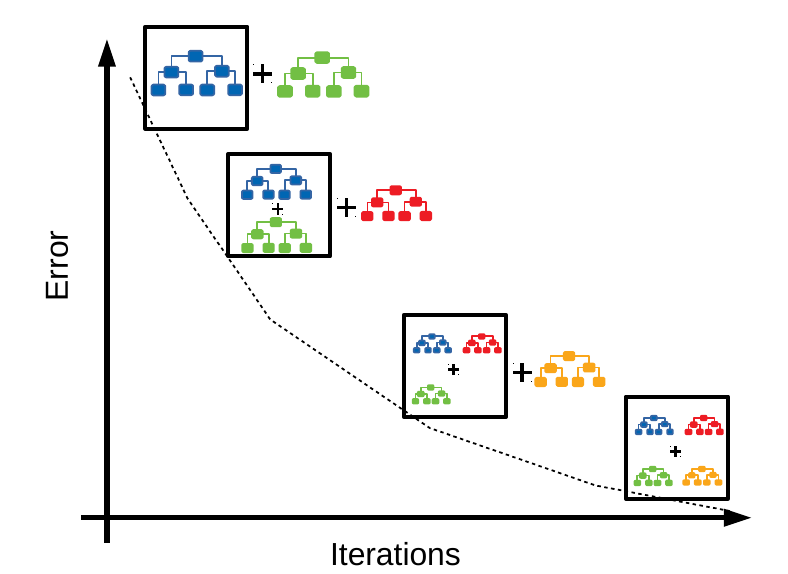
At each iteration, a new tree is added, which is trained on labels that result from the errors made by the existing ensemble of trees. In “base” boosting that would be the errors made from the ensemble, i.e. the errors of the previous iteration become the targets for the next one. In gradient boosting we train on the gradients of the errors, as determined by the loss function we are using. It’s this flexibility of choosing our loss function that makes GBTs attractive: they can be used for classification, regression, ranking, or survival analysis by simply changing the loss function we use (and its gradients).

The algorithm for growing a single tree at a high level is the following:

Until a stopping criterion is met, do the following:

1. Make predictions using the current ensemble.
2. Calculate the gradient histograms for each data point.
3. Use the gradient histograms to find the optimal split for each leaf.
4. Grow the tree by splitting the leaves.

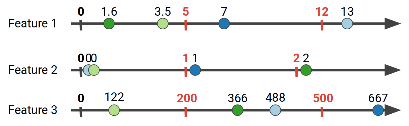
Toy Dataset

Throughout our explanation we’ll use the following toy dataset to illustrate the process:

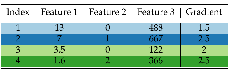
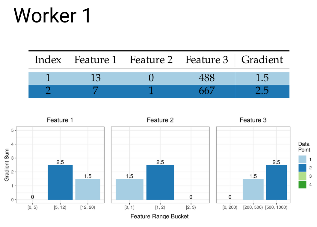
Here we have a dataset with 4 data points and 3 features, where we have also listed a gradient value for each data point.

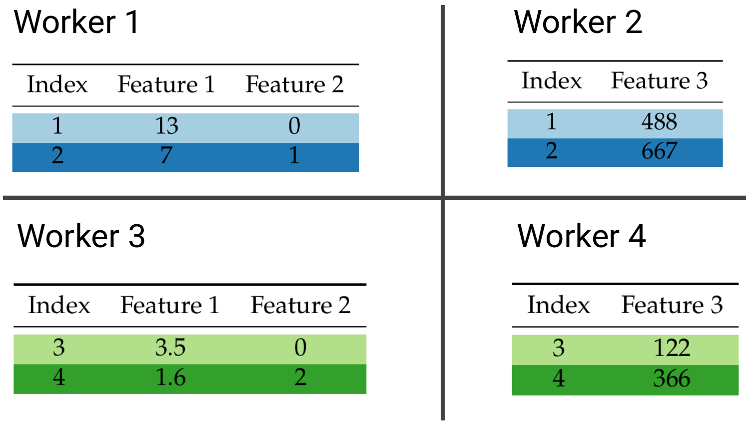
Row and block-distributed data

If you think of our dataset as a table where rows are data points and columns are features, we can distribute our data by row, column, or both. The last distribution strategy is commonly referred to as block distribution. The row and block data distribution strategies are illustrated below:

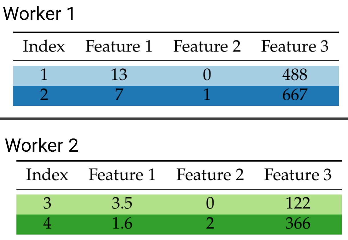
Row distributed data.

Block-distributed data.

Current state of the art implementations provide distributed GBT training using only row distribution, i.e. data are only partitioned along the data point dimension and a subset of the data end up on each machine in the cluster. Using block-distribution would allow us to parallelize learning along both dimensions, increasing the scalability of the algorithm and reducing the training cost. However, this creates a couple of additional challenges in the training process that we will expand upon now.

Prediction in the block-distributed setting

Prediction in the single-machine and row-distributed scenarios is straight-forward: For every data point we have its full features, so we can drop each data point down every tree in the ensemble and determine the exit leaf, i.e. the leaf that every data point will fall into.

The same is not the case for block-distributed data. Take for example the following tree and let’s look at data points 1 & 2:

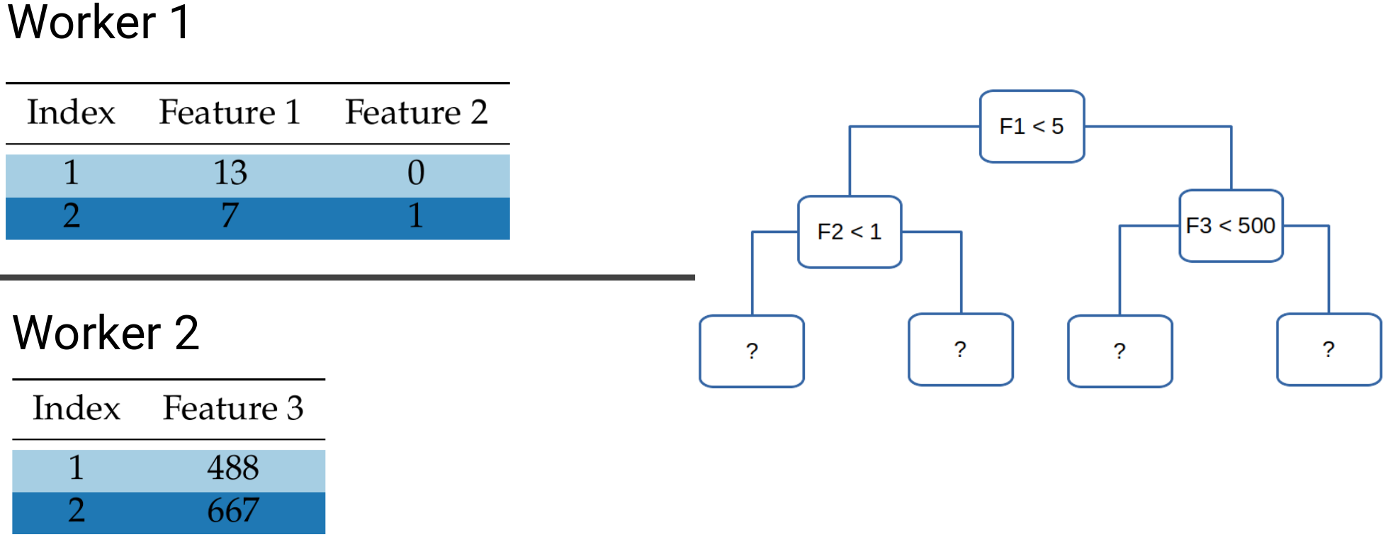
In order to determine which leafs they will fall into, we need to check the values of both Feature 1 and Feature 3. However, these lie on different workers, which means that some sort of communication is needed to determine the exit leaf. What we want to avoid is the need to communicate the data points themselves, as shuffling the entire dataset over the network would incur prohibitive network costs.

In our work we solve this by utilizing QuickScorer, an algorithm originally devised to speed up inference (prediction) in GBTs which won the best paper award in SIGIR in 2015.

Quickscorer

QuickScorer was devised to take advantage of modern computer architectures, creating a cache-friendly algorithm that uses fast, bitwise operations to determine the exit nodes in a decision tree.

The algorithm starts by assigning a bitvector to every internal node in the tree. Every bit in the bitvector corresponds to a leaf in the tree, so for a tree with 8 leaves, every internal node is assigned a bitvector with 8 bits, the leftmost bit corresponding to the leftmost leaf. Every zero in the bitvector indicates that the corresponding leaf would become inaccessible if the node evaluated to false. To determine the exit leaf for a particular data point, we take the bitvectors of all nodes that evaluate to false for that data point, and perform a bit-wise AND operation between them. The leftmost bit set to 1 indicates the exit node for the data point.

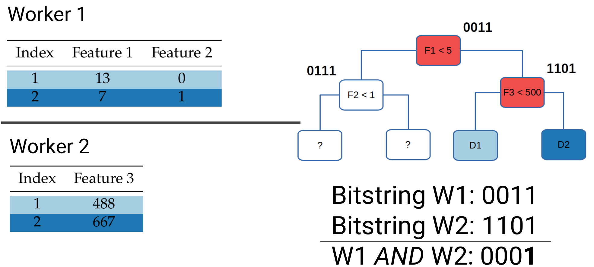
For a concrete example let’s take the data from above, focusing on data point 2, and determine which internal nodes evaluate to false:

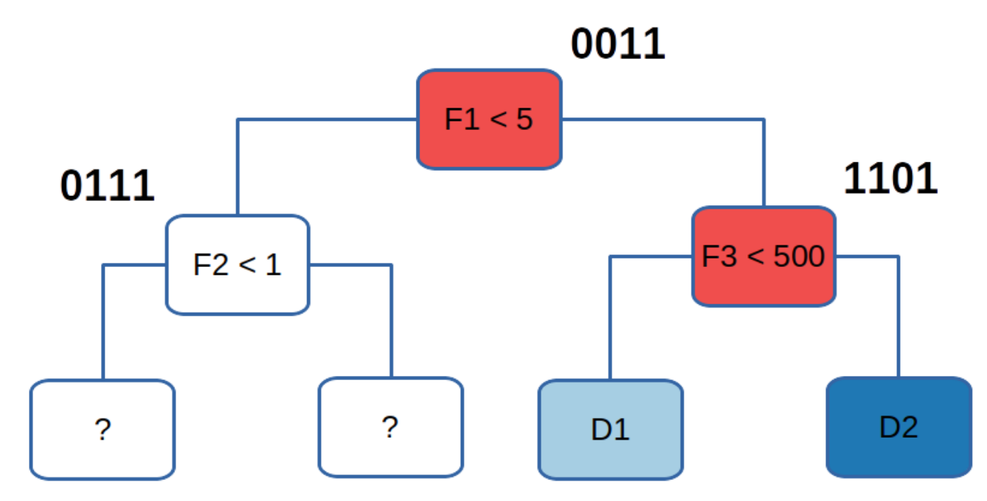
The root is given the bitvector 0011, because if it evaluates to false –assuming that we move to the right when a condition evaluates to false– the two leftmost leafs become inaccessible. For data point 2, both the root condition and the condition on the right child evaluate to false. So we would take the bitwise AND between their bitvectors, which for data point 2 would be 0011 AND 1101 which results in 0001. This means that the exit node for data point 2 is the rightmost leaf in the tree.

Block-distributed QuickScorer.

The main idea for our paper is that this evaluation of false nodes can be done independently and in parallel at each worker in a block distributed setting. Once each worker has performed their local aggregation of bitvectors, they can send them over to one server to perform the overall aggregation and determine the exit leaf for every data point. The terms server and worker are taken from the parameter server architecture we are using, explained in brief later. Briefly, worker machines store data and perform computations, while server aggregate updates and update the model.

Example of block-distributed prediction for data point 2.

Workers that share the same rows in the dataset will send their local bitvectors to the same server:

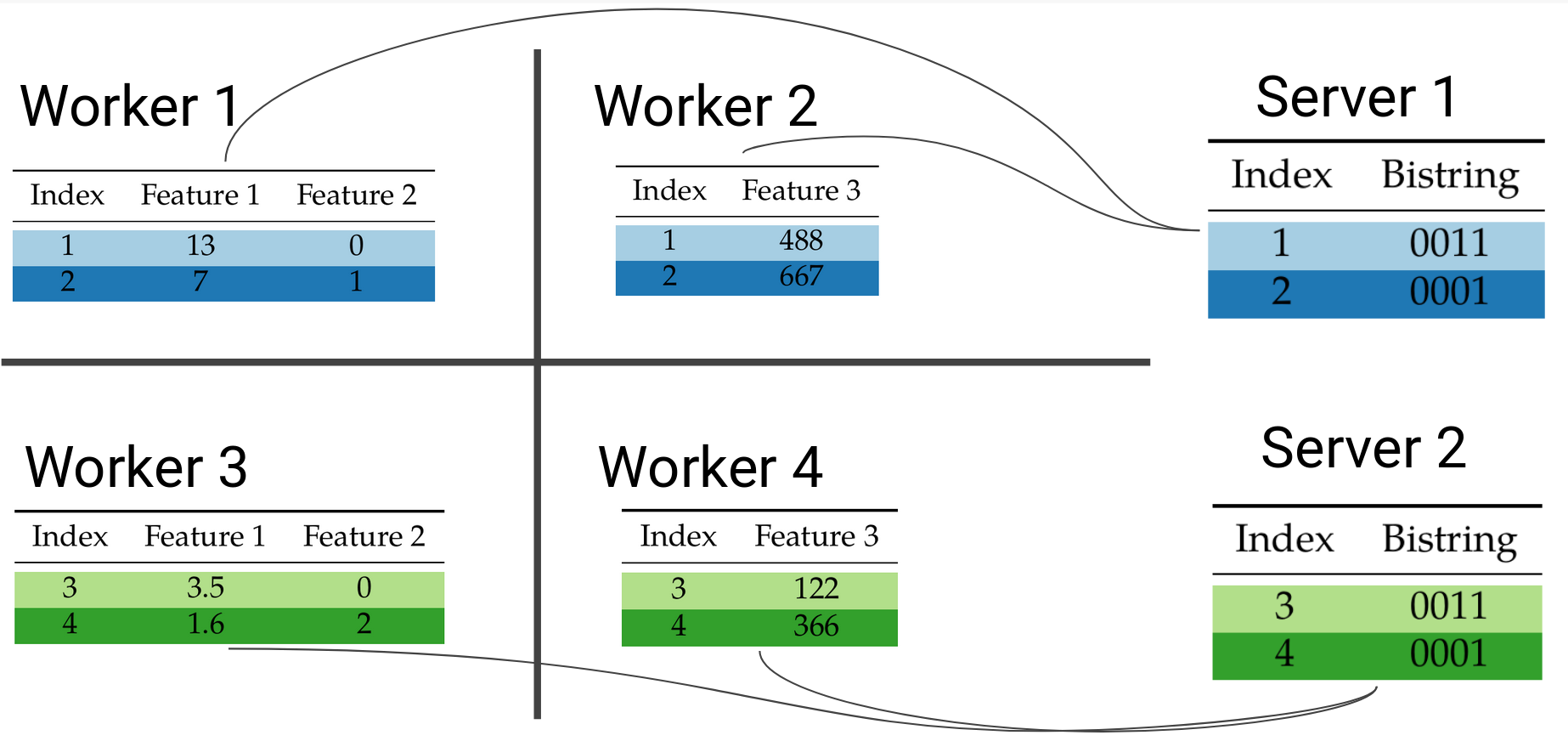
Because the AND operation is commutative and associative, the order of the aggregations and where each partial aggregation happens does not matter. The results will be provably correct as if we had done the bitwise AND locally on one machine.

Importantly, because we are only communicating lightweight bitvectors instead of the data themselves, the communication cost of prediction will be low. This solves the first problem of block-distributed learning. The second issue is how to calculate the gradient histograms and communicate them efficiently.

Calculating Gradient histograms

The most computationally intensive part of GBT learning is step 2 from the algorithm above: calculating the gradient histograms for each leaf. Gradient histograms are histograms of the gradient value of each data point, that we use to find the best split candidate for each leaf in the tree. A split candidate is a candidate for an internal node of the tree, which takes the form feature_value < threshold. In “traditional” decision trees we try to find the feature and threshold combination that allows us to best separate the data in some information theoretical sense, such as the Gini impurity. In gradient boosted trees we try to find the feature and threshold combination that provides us with the best reduction in the overall loss of the tree, which we refer to as the gain of a particular split candidate.

Gradient histogram creation

It’s best to look at this process through a concrete example.

The exhaustive way to find the optimal split point would be to take every unique feature value from the subset of data in a particular leaf and calculate the potential gain if we split on that value, for every feature.

This will quickly become computationally infeasible if we have continuous features with many (potentially billions of) unique values. What implementations like XGBoost do instead is to aggregate the gradients of specific ranges of values into buckets, to create what is called a gradient histogram for each feature.

For the data shown above, for Feature 1 we might aggregate the gradient values for the ranges of Feature 1 in [0, 5), [5, 12), [12, 20). This process is called feature quantization, and usually efficient quantile sketches are employed, such as the Greenwald-Khanna sketch. In our work we use the state of the art KLL sketch. The number of bins we choose creates a tradeoff: More bins usually mean more accuracy, but also increase the computational cost as we need to evaluate more split points, and as we will see later, increase the communication cost for distributed implementations. If we quantize all the features above, we can end up with the following bins:

The next step in the process is to take the feature bins we have created using the sketches, and aggregate the gradient values that correspond to each bin. In other words for each data point we get its gradient value according to its feature values:

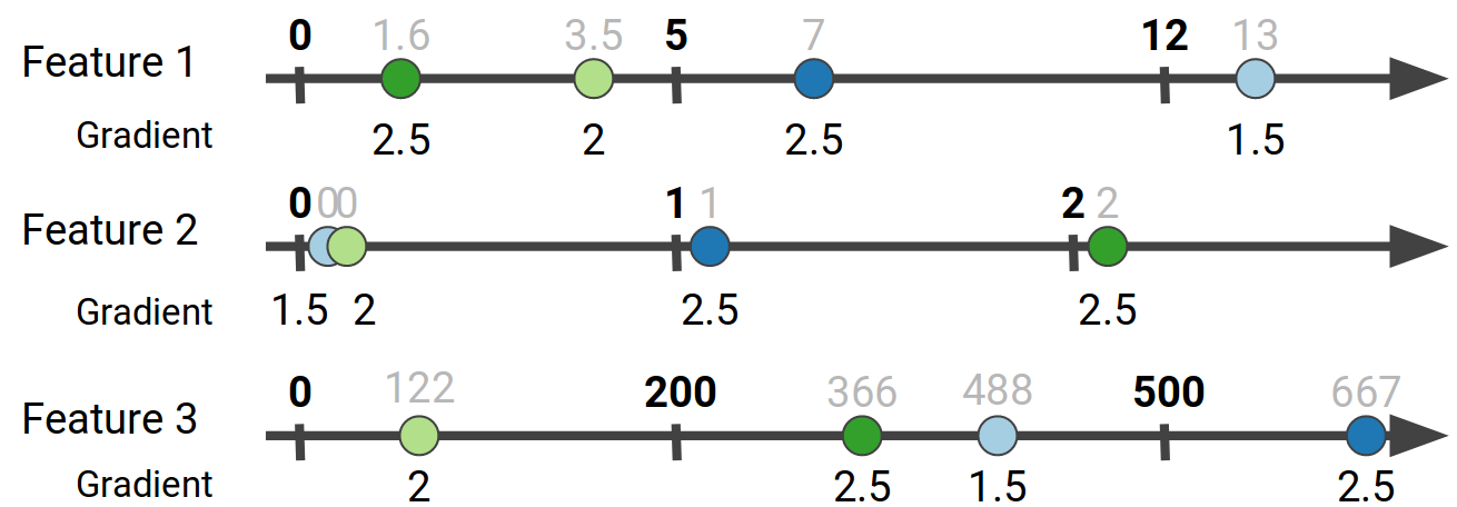
Finally we aggregate the gradient values that belong in the same bucket to get the gradient histogram for each feature:

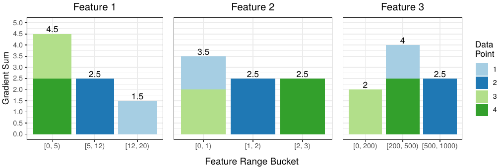
The colors help us discern the source of each data point’s contribution to a particular bucket. For example, for Feature 1, data points 3 and 4 both have values in the [0, 5) range, so their gradient values end up in the first bucket.

Split evaluation

Once we have determined the gradient histograms, we can proceed to evaluate the split candidates for each leaf. For that, we take the candidate split points for each feature, partition the data on the proposed split into the two new candidate leafs, and evaluate the potential gain in accuracy (i.e. loss reduction). The gain can be calculated by the following equation:

In the above, $g_i$ are the first order gradient values, $h_i$ the second order (hessian) gradients, and $\lambda, \gamma$ are regularization terms. $I_{L}$ and $I_{R}$ are the subsets created by splitting the subset of data points $I$ according to the split candidate to the two resulting children (Left and Right). In our simplified example we’re only using the first order gradients, and after applying a simplified version of the above equation we get the following gain values for each potential split point using the gradient histograms of the figure above:

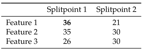
This means that if we split the data points at the Feature 1 < 5 split point, we would get the best gain in accuracy.

Row-distributed gradient histogram aggregation

The process we just described assumes that we have access to the complete dataset to create the histograms, which means that all our data should be stored in one machine¹. What happens however when our data is so massive that we need multiple machines to store it? In addition, even if we had infinite storage space on one machine, we want to be able to train our models as fast as possible, which these days means that we want to take advantage of the parallel computation. Scaling up on a single machine can be expensive and lacks fault tolerance, so often we employ clusters of commodity computers to quickly and reliably train models on massive data.

When data are row-distributed we have two challenges to solve: The first one is creating the feature quantiles that give us an estimate of the empirical cumulative distribution function for each feature. These are then used to create the so called gradient histograms that allows us to determine the best way to grow our tree. The problem arises from the fact that each worker only has access to a subset of the complete dataset, which makes communication for both of these steps necessary.

Mergeable quantile sketches

Determining the quantile sketches is relatively straightforward: some quantile sketches have the property that they are mergeable: given a stream of data, applying the sketch to parts of the stream and then merging those partial sketches will have the same result as if we had applied the sketch to complete stream. This means that we can create partial sketches at each worker, and then merge those sketches to get the complete feature quantiles. This requires communicating the partial sketches over the network. More on the potential issues with that will come later.

Communicating partial gradient histograms

Similarly to how we can create partial quantile sketches, we can also create partial gradient histograms that then need to be merged to create the overall histogram for each leaf. Once we have the buckets from the previous step we can create the local histograms at each worker:

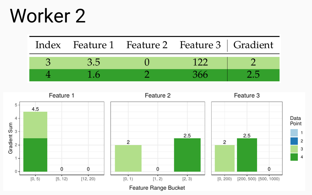
These then need to be communicated between the workers so that all workers end up with the same copy of the merged gradient histograms. See all those zeros that have now appeared in our histograms? This is the cause of the issues in the current state of the art.

Issue with the state of the art: Dense Communication

The problem with the above approach is that all current implementations utilize some sort of an all-reduce operation to sync the sketches and histograms between the worker. In short, an all-reduce operation will apply an aggregation function to each element in a vector, and then make the aggregated result available to each worker in the cluster. In the following example we have 4 vectors which we want to aggregate element-wise, using addition as our aggregation function.

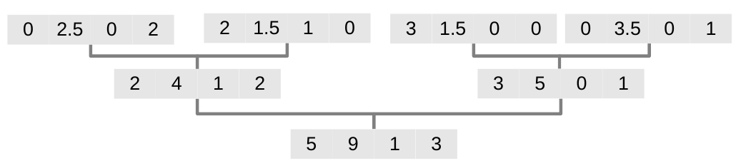All-reduce aggregation of vectors. The final result is propagated back from the root to every node in the tree.

All² (like MPI) current all-reduce implementations use dense communication to perform this operation. This means that the number of elements to be aggregated needs to be known in advance, and each element must have the same byte size.

Why is this a problem? In the simple vector aggregation example given above, almost half the elements are zeros. Because of this system limitation, every vector being communicated will need to have the same byte size, regardless of the number of zeros in it. This causes a lot of redundant communication. Similarly to the vectors in this example, the gradient histograms are also sparse, as we can see with the example for Workers 1 and 2 further up. As we increase the number of buckets and the number of features, that can be in the millions or billions, the amount of zeros being communicated will increase, creating massive unnecessary overhead. It this problem in particular that we attack with our approach.

Block-distributed gradient histogram aggregation

Our idea to deal with the problem is to communicate sparse representations of the histograms. Sparse representations can be thought of as maps that compress the size of vectors and matrices with a high ratio of zeros in their values. That requires a communication system that can deal with different workers communicating objects with different byte size. As we mentioned above, systems like MPI do not allow us to communicate objects of arbitrary size.

Another communication system with a more flexible programming paradigm is the Parameter Server (PS). In this system, every machine in the cluster assumes a particular role: Servers are responsible for storing and updating the parameters of the model. Workers store the training data and are responsible for the computation of the updates to the model, which they then forward to the servers. Importantly, the parameter server allows point-to-point communication between servers and workers, allowing each worker to send over objects of arbitrary size, making it a perfect candidate for sparse communication. DimBoost (paywalled) was the first paper to use the PS for GBT training and served as an inspiration for our work. However, DimBoost still uses dense communication.

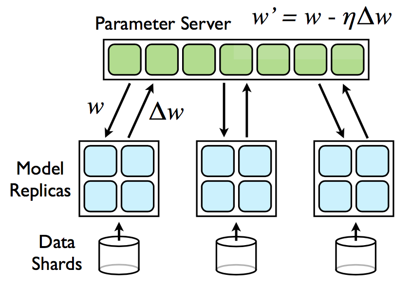
Source: Google DistBelief

In our work we represent the gradient histograms as sparse CSR matrices, each row corresponding to a feature, and each column to a bucket in the histogram. Each worker populates its own sparse matrix, and then sends them over to one server. Each server is responsible for creating the gradient histograms of a specific range of features, so the workers that are responsible for the same sets of features will send their histograms to the same server.

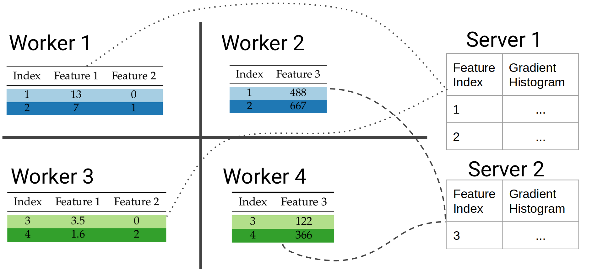
In the example above, Server 1 is responsible for features 1 and 2, and Server 2 for Feature 3. The workers that share the same columns of data will send their partial histograms to the same server. Each server can then aggregate the partial histograms, and calculate the best local split candidate from its local view of the data. It takes one final communication step to determine the best overall split candidate.

Results

So how much difference in terms of communication can this strategy make? To test our hypothesis, we implemented both versions of the algorithm in C++, basing our code the XGBoost codebase that makes use of the rabbit collective communication framework. For our parameter server implementation we use ps-lite.

To test the performance of each method under various levels of sparsity we used 4 datasets for binary classification, taken from the libsvm and OpenML repositories. URL and avazu are two highly sparse datasets with 3.2M and 1M features respectively. RCV1 is less sparse with 47K features, and Bosch is a dense dataset with 968 features.

We use a local cluster of 12 workers, using 9 workers and 3 servers for the block-distributed experiments, and all 12 machines as workers for the row-distributed ones. We measure the communication cost of each approach by the size of the histograms created by each method, measured in MiB. We also measure their real-world performance as the time spent in communication and computation during histogram aggregation.

Byte size of the gradient histograms

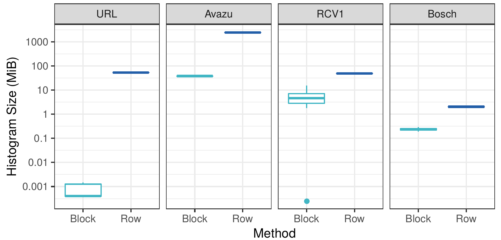
In the figure above we can see that our block-distributed approach creates histograms that are several orders of magnitude smaller than the dense row-distributed method. This confirms our hypothesis that for sparse datasets there are massive amounts of redundant communication in current implementations.

Communication-Computation time

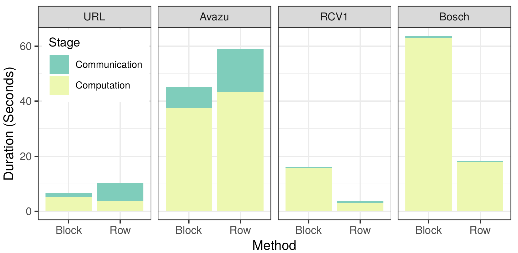
The figure above shows us the time spent communicating data and performing computation for each approach. For the sparse datasets URL and avazu, we can see a large decrease in the time required to communicate the gradients, and a modest increase in computation time that leads to an overall improved runtime. However, for the more dense datasets the difference in communication time is small, while the computation time increases significantly. This is caused by the overhead introduced from building the sparse data structures, which, unlike the dense arrays used by the row-distributed algorithm, are not contiguous in memory and require constant indirect memory accesses. This, in addition to the overhead introduced by the parameter server, lead to an increased overall time to compute the gradient histograms for the dense datasets.

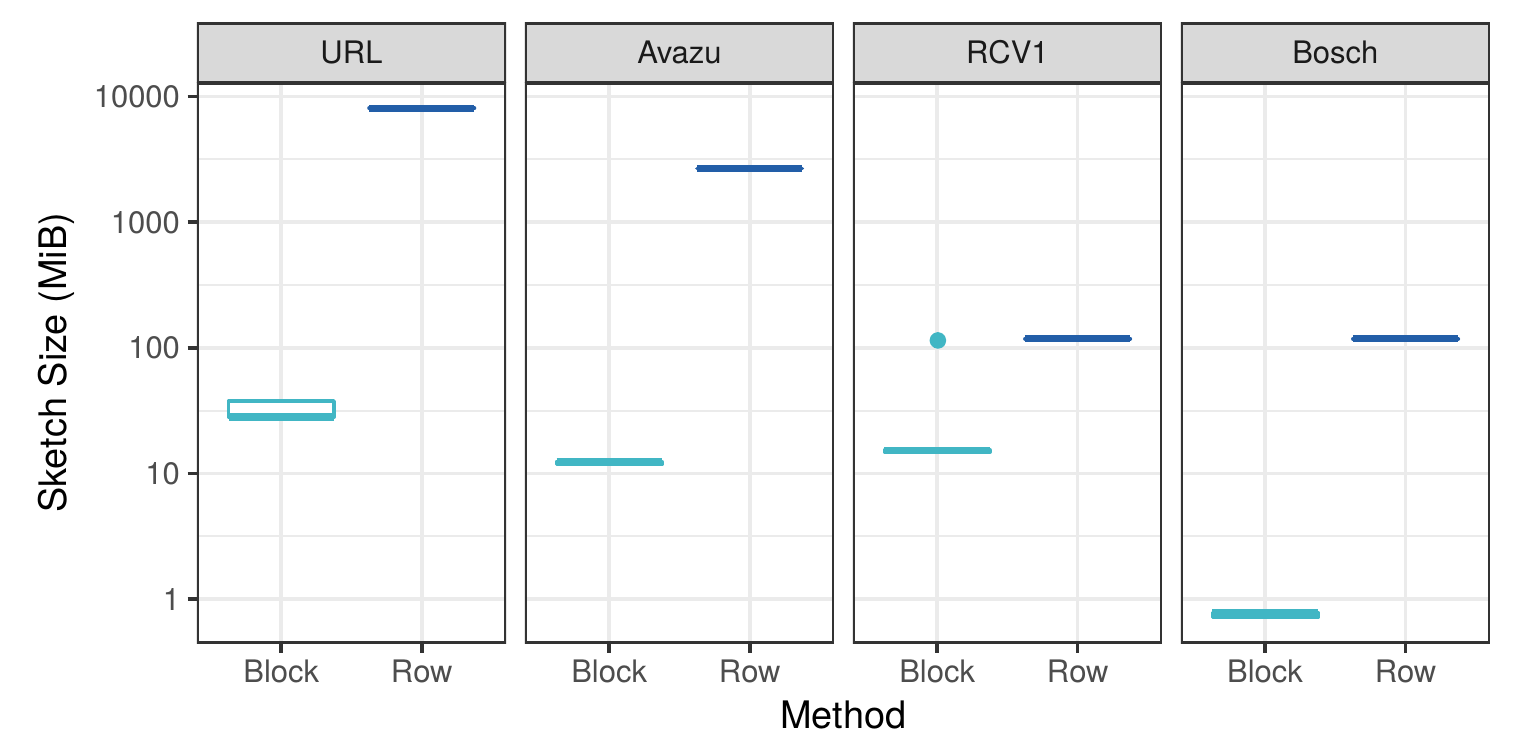
Quantile sketch size

Another aspect where dense communication can significantly increase the cost are quantile sketches. As we mentioned above, in order to determine the ranges for the buckets in the gradient histograms, we need an estimate of the cumulative density function for each feature. This is done in the distributed setting by creating a quantile sketch at each worker, and then merging those to get an overall quantile sketch.

The issue with dense communication of quantile sketches is that these are probabilistic sketches, and as such their actual size cannot be known in advance. What systems like XGBoost have to instead is to allocate for each sketch the maximum possible size it can occupy in memory, and communicate that. For such efficient quantile sketches the maximum theoretical size can be multiple orders of magnitude larger than the sketch’s actual size. Using our approach we are able to just communicate the necessary bytes, and not the theoretical maximum for each sketch, leading to massive savings:

As shown in the original XGBoost paper (Figure 3), being able to communicate the sketches at every iteration instead of only at the start of learning (local vs. global sketches) leads to similar accuracy with fewer bins per histogram, enabling even more savings in communication.

Conclusions

In this work we demonstrated the value of sparse communication, and provided solutions for the problems that arise with block-distributed learning. Using a more flexible communication paradigm we are able to get massive savings in the amount data sent over the network, leading to improved training times for sparse data.

This works opens up avenues for plenty of improvements. First, while we have created a proof-of-concept system to evaluate the row vs. block distribution in isolation, the real test will come by integrating these ideas in an existing GBT distribution like XGBoost and evaluating its performance in a wide range of datasets against other state-of-the-art systems like LightGBM and CatBoost.

In term of the algorithm itself, one easy improvement is the use of the RapidScorer algorithm in place of QuickScorer that uses run length encoding to compress the bitvectors for large trees. Such a method can bring further communication savings for prediction.

If there’s one takeaway for users and especially developers of GBT learning systems is that current communication patterns are highly inefficient, and massive savings can be had by taking advantage of the inherent sparsity in the data and intermediate parts of the model like the gradient histograms. This, in addition to the new scale-out dimension that block-distribution enables, can make distributed GBT training even cheaper and efficient.