Uncovering similarities and concepts at scale
I defended my thesis recently and finally have some time to look back to look over the work I’ve done the past few years from a distance. Over the next few weeks I’ll be going over each of the papers included in my dissertation, to present them in a more accessible format.
This first post is about a scalable way to determine similarities between objects and grouping them in coherent groups. We’ll give examples of how we’re able to combine deep learning with graph processing to uncover “visual concepts” along with an high-level explanation of the algorithm. The code for this work is available on Github.
Introduction
Finding similarities is one of the fundamental problems in machine learning. We use similarities between users and items to make recommendations, we use similarities between websites to do web searches, we use similarities between proteins to study disease etc.
So a natural question that comes up is: how can we efficiently calculate similarities between objects? There have been many approaches for this purpose proposed in different domains, like word embeddings, collaborative filtering, and similarity learning. Once we have calculated similarities between objects, how can we then discover groups of objects that belong together?
In this post I will provide an overview of our work on scalable similarity calculation and concept discovery presented at ICDM 2015 and extended in our KAIS paper, in which we model objects as nodes in a graph where the edges represent similarities between objects. I will show how one can create correlation graphs from data, and how one can transform that graph to extract similarities between objects, and finally how we can use the similarity graph to create interesting groups of similar items which we call concepts, with illustrative examples.
This post will be a bit long so you can skip ahead to the section that interests you most:
- Introduction
- Creating the correlation graph
- Transforming the correlation graph into a similarity graph
- Uncovering concepts
- Examples
- Conclusion
Problem description
Our problem description is this: Given a dataset that we know encodes some relations between our objects, how can we calculate similarities between objects that interest us? And how can we do that in scalable manner, if we assume we have potentially billions of records to learn from?
Our algorithm should have a few characteristics that make it attractive:
- Accurate: Clearly we want our resulting similarity scores to make some kind of sense in our domain. If we are calculating similarities between music artists, we would like our score to assign high similarity between the Wu-tang Clan and Nas, but low similarities between Wu-tang and Tchaikovsky.
- Domain Agnostic: We would like our algorithm to be applicable in various domains, rather than being specialized in one. For example while collaborative filtering works well in determining similarities between users and items, given a user-item interaction matrix, it’s not intuitive to apply it in order to obtain similarities between proteins.
- Unsupervised: We want our algorithm to be able to discover similarities based on relations that are present in the source data in an unsupervised manner. Relying on human-curated databases like WordNet brings with it many problems like slow adaptation of new terms, limited coverage and most importantly, high cost.
- Scalable: Relying on data to uncover similarities means that we should be able to use very large datasets that could contain latent information about the relationships between our objects. If our algorithm scales unfavorably with the amount of input data, we would have to rely on subsampling, potentially losing useful information about the interactions between the objects.
Our Approach
In order to achieve these desiderata we decided to take a two step approach: We first process our dataset to create a compact representation of it we call the correlation graph. This graph can include some useful relationships, but can also include spurious correlations. Take for example the words “Messi”, who is a famous footballer, and “ball”. These will often appear within a short distance in text, meaning they are correlated. This however does not mean that Messi is similar to a ball! We want to have a method that allows us to discover deeper semantic relationships between objects and not just correlations.
For that purpose, we further transform the correlation graph into a similarity graph. The similarity graph should capture semantic relationships, and we focus on exchangeability of an object. If we take the word “Messi” in a sentence and replace it with Ronaldo, the sentence should still make sense. Ideally we would like our algorithm to be able to group Messi and Ronaldo in the same semantic group.
We call these semantic groups “concepts” and our approach to uncovering them is to apply a community detection technique on top of the similarity graph.
The focus of our work and of this post will be on the transformation between correlation and similarity graph; of course choosing how to create the correlation graph and perform community detection are of great importance, so we will show a couple of examples we used that should be applicable in various settings.
Graph-based vs. vector-space similarity
You might have noticed that we have mentioned two approaches to calculating similarities that are quite different: Graph-based similarity and vector-space similarity which is used in, for example, word embeddings.
The overall idea in vector-based similarity is to embed objects in some vector space and then use distance measures like Euclidean or cosine distance to measure their similarities. This approach has proven to work well in a number of fields; apart from the ones we have mentioned above RNN word embeddings have been very successful in the NLP field. Concept discovery is done in this case using traditional clustering techniques like kMeans clustering.
There are however some problems with this kind of approach. Since these are usually iterative methods they tend to be computationally costly, as they require multiple passes over the complete dataset to converge. They also tend to have parameters that significantly affect their performance that can be hard to tune without the use of expensive cross-validation, such as the number of factors to use in a matrix factorization technique, or the dimensionality of the embeddings.
By using a graph representation instead, the connections between objects arise from the data themselves, and this allows us to discover higher-order structures and relationships between objects in an efficient manner, all while having compact representation of the data. Importantly, we only require a single pass over the data to create the correlation graph, and provide a scalable algorithm for the similarity transformation.
Creating the correlation graph
The correlation graph would usually be created from data, unless you already have access to a model of correlations between objects, like the codon substitution matrix we used as an example in our paper.
The creation of the correlation graph is a very important step in the whole process, as the “garbage in, garbage out” principle holds very true in machine learning. If we want our similarity graph to be meaningful, the correlation graph should encode some information about the relationships between objects. Fortunately it’s relatively straightforward to create a correlation graph for two of the most important types of data on the web: text and user interaction data.
For these types of data one can simply model objects as nodes and some measure of co-occurrence between objects as the edges between them. For example one could create one node in the graph for each word in the dataset, and create edges between words weighted by their conditional probability, e.g. how probable is it that we will see the word “dog” given that we have observed the word “cat” within a sentence? Or in the case of user data, what is the conditional probability of a user interacting with item A given that he has interacted with item B?
If we extract a (compactly represented) co-occurrence matrix, we are then able to create many different correlation graphs, by choosing a different correlation measure. For text we obtained the best results using pointwise mutual information but one could also use a multitude of other measures like, the Jaccard Index or the Sorensen-Dice coefficient among others.
One can imagine using similar approaches for other types of data, so the above is not limited to text and user data. In the examples below we will show how one can use a combination of supervised deep learning and our method to uncover visual concepts.
Transforming the correlation graph into a similarity graph
Creating the correlation graph should generally be a straightforward process. But, as mentioned above, the correlation graph will not necessarily model the kinds of relations we want to capture. We are aiming for semantic similarity, not simple correlation.
In order to discover similarities then, we follow the popular addage by J.R. Firth’s:
“You shall know a word by the company it keeps.”
Our goal is to extend this definition and talk about any object, not just words. The way we do this is by looking at the neighborhood (or context) of the items and calculating a similarity score based on the similarity of their contexts.
The central element of out approach is the correlation-to-similarity graph transformation. The main idea is to assign higher similarity to nodes whose contexts are themselves similar. Nodes that have strong correlations to the same nodes, and little other correlations will be assigned higher similarity themselves. In the example correlation graph below, we are interested in calculating the similarity between nodes 4 and 7. The weight of the correlation is indicated by the width of the edges. Nodes 4 and 7 have strong correlations to the same set of nodes (2,3,5,6) and few weak correlations to other nodes. Since their “contexts” are similar, we posit that the nodes themselves should be similar. The exact calculation is given below, as well as in the paper, but hopefully this provides enough intuition.
 An example correlation graph. Nodes 4 and 7 have similar contexts,
so should be similar themselves.
An example correlation graph. Nodes 4 and 7 have similar contexts,
so should be similar themselves.
In order to achieve scalability we take into consideration only two-hop neighbors in our calculation. While this may seem limiting at first, it allows us to uncover deep relationships as we will see in our examples. Based on this approach we can take any correlation graph and transform it into a similarity graph as shown here:
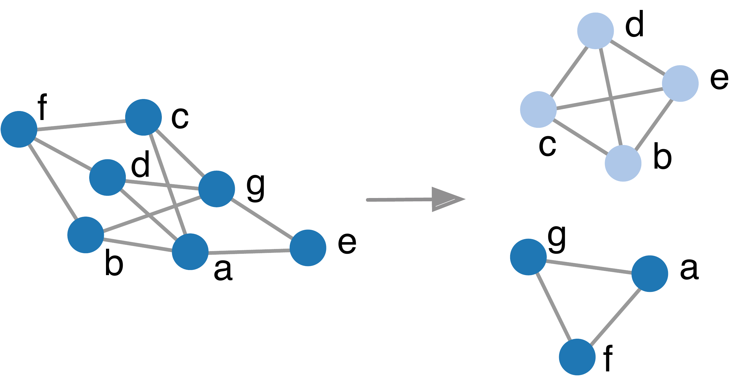 An example of a graph transformation, from a correlation graph into
a similarity graph.
An example of a graph transformation, from a correlation graph into
a similarity graph.
Math
Time for some math and definitions taken from our paper then. If you’re not interested in these feel free to skip to the examples. The TLDR is that we sum the correlations of every two-hop neighbors, calculate how much they have in common vs. uncommon and determine their similarity as a result of that.
Let $C = {i}\und{i=1}^n$ be a set of objects, where each object has a correlation, $\rn{i,j}$, to every other object. The context of an object $i$ are its relations to all other objects, $\rn{i} = (\rn{i,j})\und{j=1}^n$.
The way we define we define the similarity $\sy{i,j}$, is by subtracting the relative $L\und1$-norm of the difference between $\rn{i}$ and $\rn{j}$ from 1; that way we transform a difference measure to a similarity measure:
\[\begin{equation}\label{eq:sim} \sy{i,j} = 1 - \frac{\dnm{i}{j}}{\rns{i} + \rns{j}}, \end{equation}\]where
\[\begin{equation}\label{eq:totrel} \rns{i} = \sum\und{k \in C} | \rn{i,k}| \end{equation}\]and
\[\begin{equation}\label{} \dnm{i}{j} = \sum\und{k \in C} | \rn{i,k} - \rn{j,k} |, \end{equation}\]denoted $\nm{i,j}$ for short.
In order to make the computation scalable, we only calculate similarities between items that are one-hop neighbors in the graph, that is, in order for two items to have a similarity score in our approach they must share at least one common neighbor. We can then define $\nm{i,j}$ as:
\[\nm{i,j} = \rns{i} + \rns{j} + \Lambda\und{i,j},\]where
\[\begin{equation} \Lambda\und{i,j} = \sum\und{k \in n\und{i} \cap n\und{j}} (|\rn{i, k} - \rn{j, k}| - |\rn{i, k}| - |\rn{j, k}|) \label{eq:l1common} \end{equation}\]In the paper we provide more details about how to make the approach scalable, namely applying a max in degree for nodes and a weight threshold for the edges, motivated by the observation that most items in the graph are unrelated, so we should avoid including in the computation small, potentially spurious correlations.
Uncovering concepts
We mentioned earlier that the notion of a concept in a similarity graph lies in the graph structure, i.e. communities or clusters are encoded in the way that nodes are connected with each other. The equivalent of clustering in a vector-space is commonly referred to as community detection in the graph literature.
Community detection is a heavily researched topic, and I encourage you to take a look at this excellent survey by Santo Fortunato for an overview of the field. In the context of this work we wanted a community detection that was scalable and ideally allowed for overlapping communities. Overlapping community detection aims at assigning nodes to one or more communities, as most objects in the real world belong to more than one community. A person for example might belong to a group of friends, a (potentially overlapping) group of colleagues, a gym club etc. Uncovering such communities is computationally challenging, but some very interesting algorithms have recently been proposed, like the one from Yang and Leskovec, and you can take a look here for an overview of the area.
In our work we used a variant of the SLPA algorithm. SLPA is a community detection algorithm based on label propagation that can scale to graphs with millions of nodes and billions of edges. It is an iterative algorithm where each node maintains a memory of community labels that are exchanged over the edges of the network. Nodes will sample from their incoming labels and maintain the most frequent ones in their memory. As we move from iteration to iteration, the memory of each node will gradually converge to a small subset of labels, which are used to label each node with overlapping communities.
 An example of community detection.
Examples
Now that we’ve seen how the method works let’s take a look at the kinds of output that is possible using this approach. We’ll look at examples from the text and image domains, where in the latter we combine the power of supervised deep networks with our algorithm to uncover visual concepts.
Text
The first example comes from the Billion word corpus which is a standardized dataset originating from crawling news sources. As such, the concepts uncovered relate to the words that commonly appear in news sources.
Here we have used the probability of co-occurrence within a window of 2 (bigrams) between two words to create the correlation graph, then applied our transformation to get the similarity graph from which we are then able to uncover concepts.
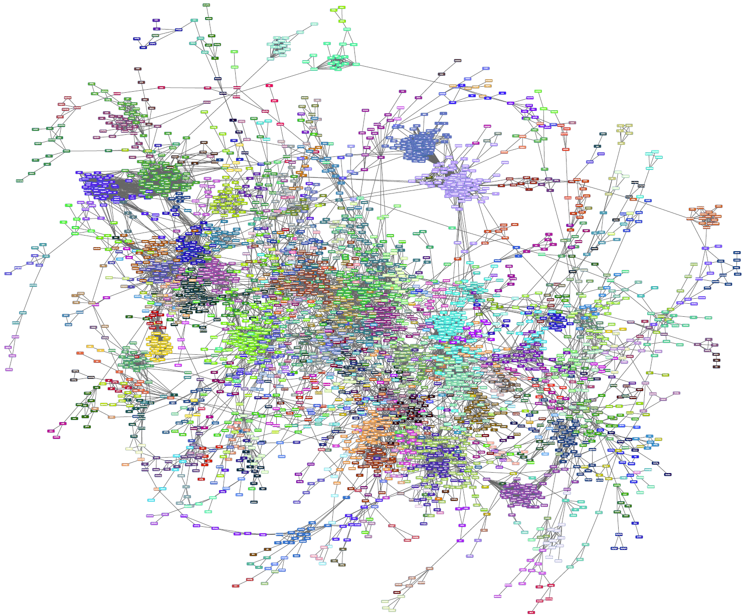
The full graph is shown at the top of this page and the zoomable PDF file is also available. Here, we’ll zoom into a couple of interesting regions of the graph to demonstrate the kinds of concepts we are able to discover.
People
In the first example we can see concepts of names being grouped together. On the left we have names of political figures like Blair, Clinton, and Obama. On the right we have names of athletes being grouped together, like Favre, Williams, and Armstrong.
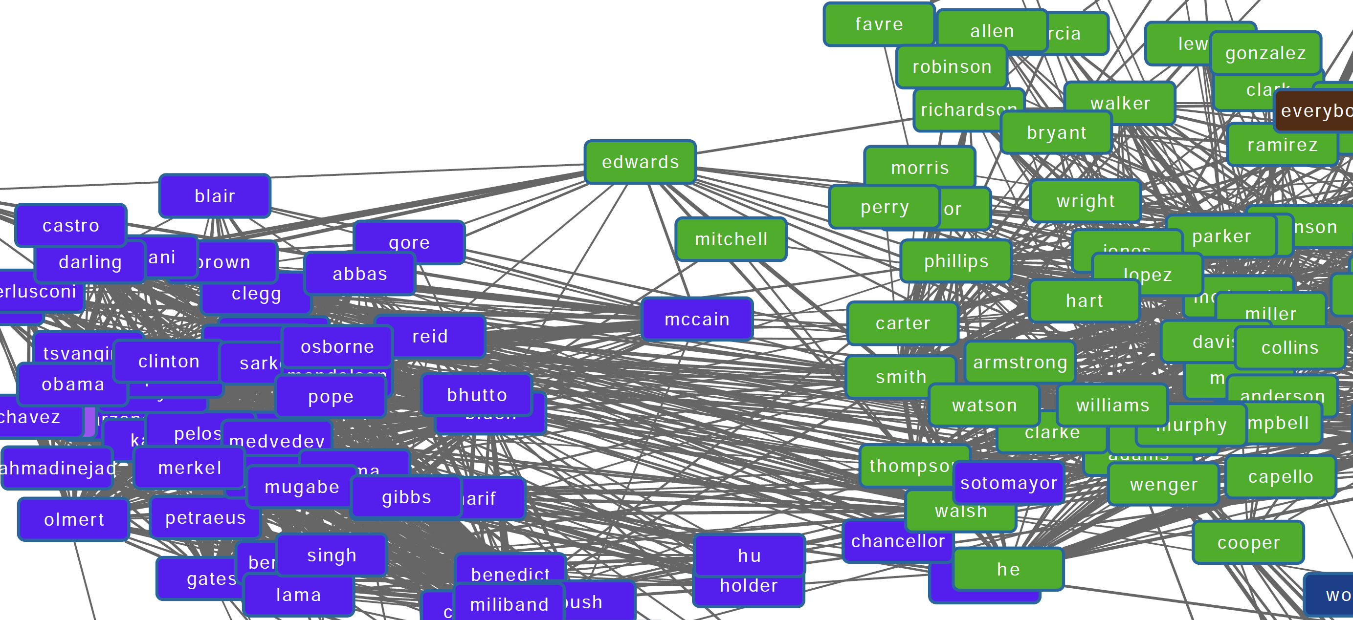 Two uncovered concepts of names: politicians on the left, and athletes on the right.
Nationalities & Groups
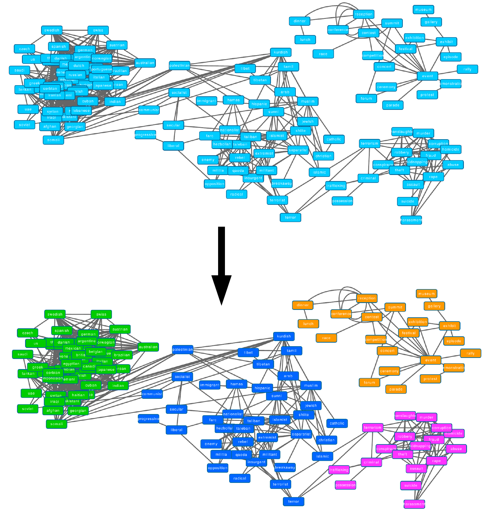
In this second example we can see one group of nationalities uncovered, which in turn connects (as we move to nationalities that commonly appear in the news like Palestinian, Kurdish, and Tibetan) to groupings of people, including religions and organizations that are likely to appear in the news.
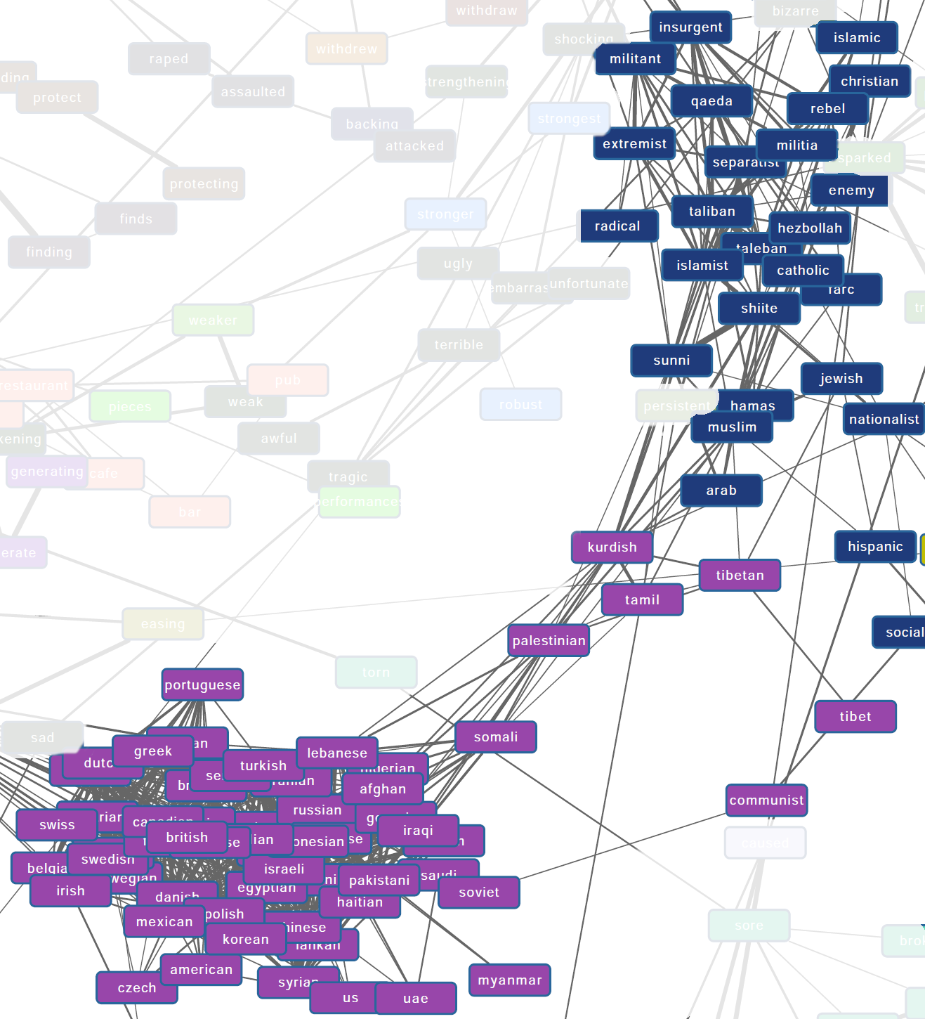 These concepts group together nationalities on the left and other groups on the right.
Visual Concepts
For the next example we combine the power of supervised neural networks with our unsupervised learning algorithm to uncover concepts from raw images. Deep neural nets can be trained on a large labeled dataset like ImageNet to recognize thousands of objects in an image. We can then use the trained network on millions of unlabeled images to generate approximate labels. Using those labels, we can create a correlation graph and apply our algorithm to uncover what we call “visual concepts”.
In this example we use the OpenImages dataset released by Google that has annotations for approximately 9 million unlabeled images from the Flickr image hosting service. These images were annotated using a collection of neural network models with 19,995 classes in total, with image being annotated with 8.4 labels on average.
Forming the correlation graph.
To create the correlation graph we create a clique (fully connected graph) for all the labels that appear together in a single image. As objects appear together in the real world these cliques are then connected to other cliques, forming the full correlation graph.
We give an example in the following figure: Here we have two annotated images of people in cowboy hats. In the top image, the neural network has missed the person label, and the human face label, because it is obstructed by the hat. When we create the correlation graph however, the guitar label is connected to the person as a second degree connection, so given enough data, we can deduce that guitar appears often in the context of person.
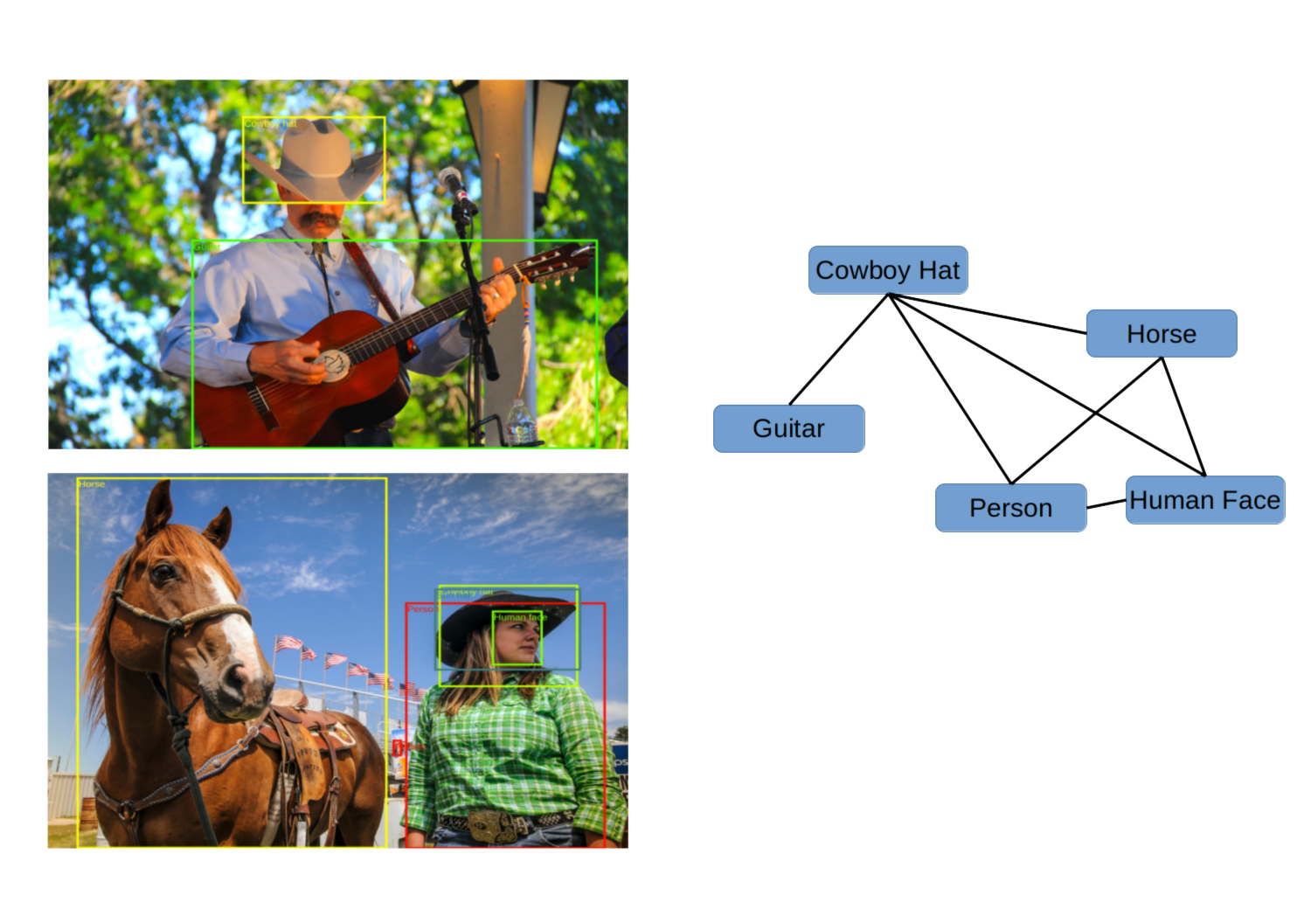 Creating the correlation graph from the OpenImages annotations.
Example concepts
After creating the correlation graph as described above, we can apply our transformation and create the visual concepts, a couple of examples of which we give here. You can view the full visual concept graph here.
As expected from images taken from the Internet, we have concepts of cats and dogs, with various breeds being grouped together, and another concept with species of birds (in orange):
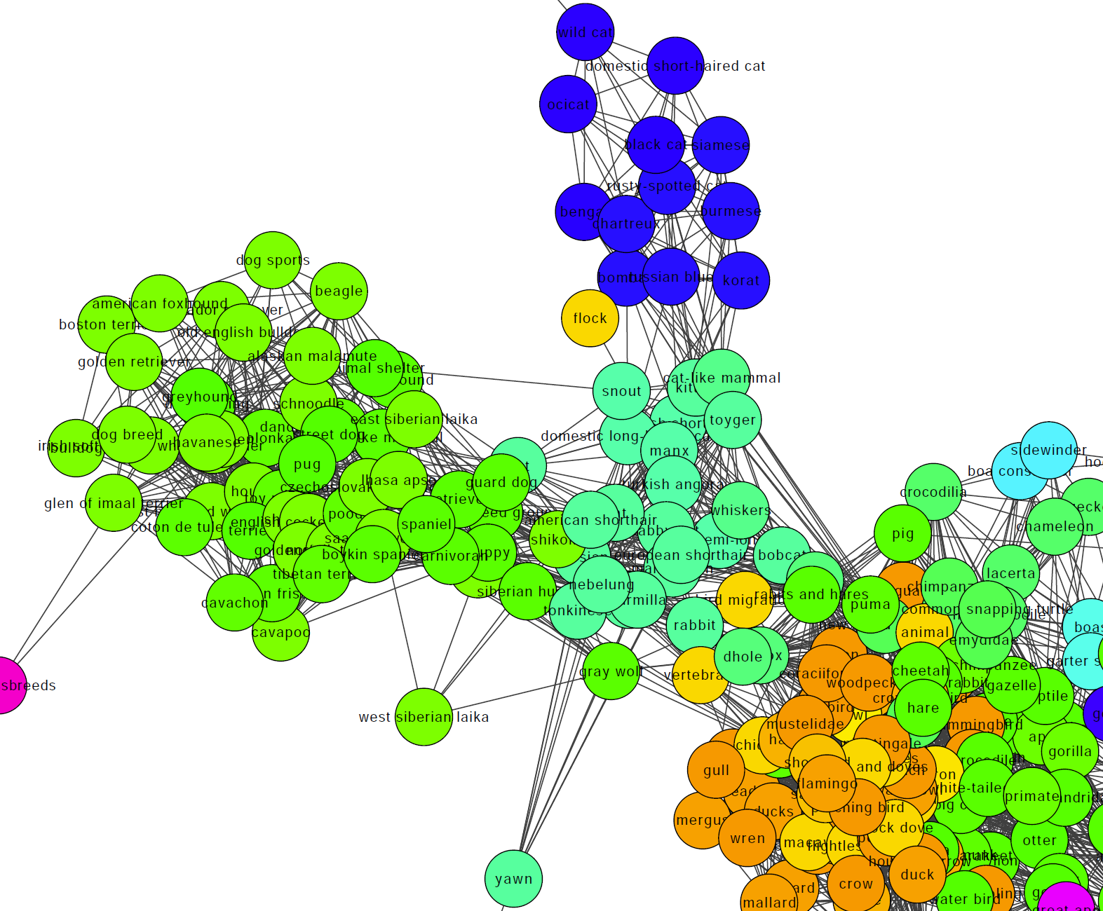 Animal concepts uncovered from real-world images.
In another example concept we have various sports being grouped together, with a contact sports concept forming on the right.
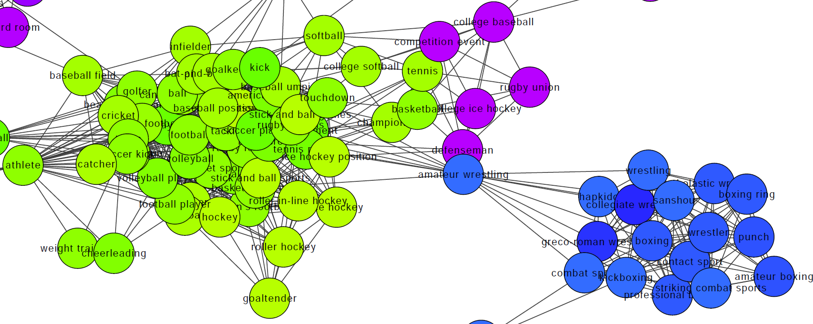 Sports concepts uncovered from real-world images.
We can see then the potential of combining the two methods: It provides a new lens into the world, extracted from real world images. This can provide us with insights that are not present in text corpora.
Conclusion
In this post we described how we can calculate the similarities between objects in any domain, provided that we have access to a set of approximate correlations between them. Using the generated similarity graph we can then group objects in coherent clusters which we call “concepts”, allowing us to discover structure and knowledge from large-scale unlabeled data.
In the paper we provide more details showing a quantitative evaluation vs. word embedding methods and demonstrate the scalability of the approach by training on the Google N-grams dataset (24.5 billion records) in a matter of minutes.
Discussion - Links to posts on social media
As mentioned before, the code is available on Github.